Imaging Overview
JACAL Architecture
JACAL is a package in which elements of Yandasoft have been extracted from their MPI-based framework and reset within DALiuGE. The current level of granularity of imported code is one level down from the Yandasoft imaging applications, with separate DALiuGE drops for major cycles (visibility inversion and prediction) and minor cycles (image based deconvolution). At lower levels the Yandasoft libraries are used, and at higher levels DALiuGE is used. As described below, recent updates have added an extra level of control at the major cycle level, with separate drops for visibility ingest, inversion and prediction. This will become the standard level used in JACAL going forward.
Standard Yandasoft continuum imaging has visibility inversion and prediction tasks partitioned across a cluster, with different MPI ranks handling one or more spectral channels and/or Taylor terms. A range of gridders and degridders are available for these tasks. After prediction, subtraction and inversion, the intermediate images are merged to a single MPI rank for joint image-based preconditioning and deconvolution. Such a setup can also be achieved in JACAL by expanding the example graph from the EAGLE Usage section. For example, the following graph generates dirty and PSF images separately for four spectral channels, which are then reduced (merged) into a single set that are passed to the solver for deconvolution. The output clean-component sky model is distributed to another set of major cycle components for visibiltiy prediction, subtraction and inversion, and the resulting residual images are again reduced to a single image for restoring and then output.
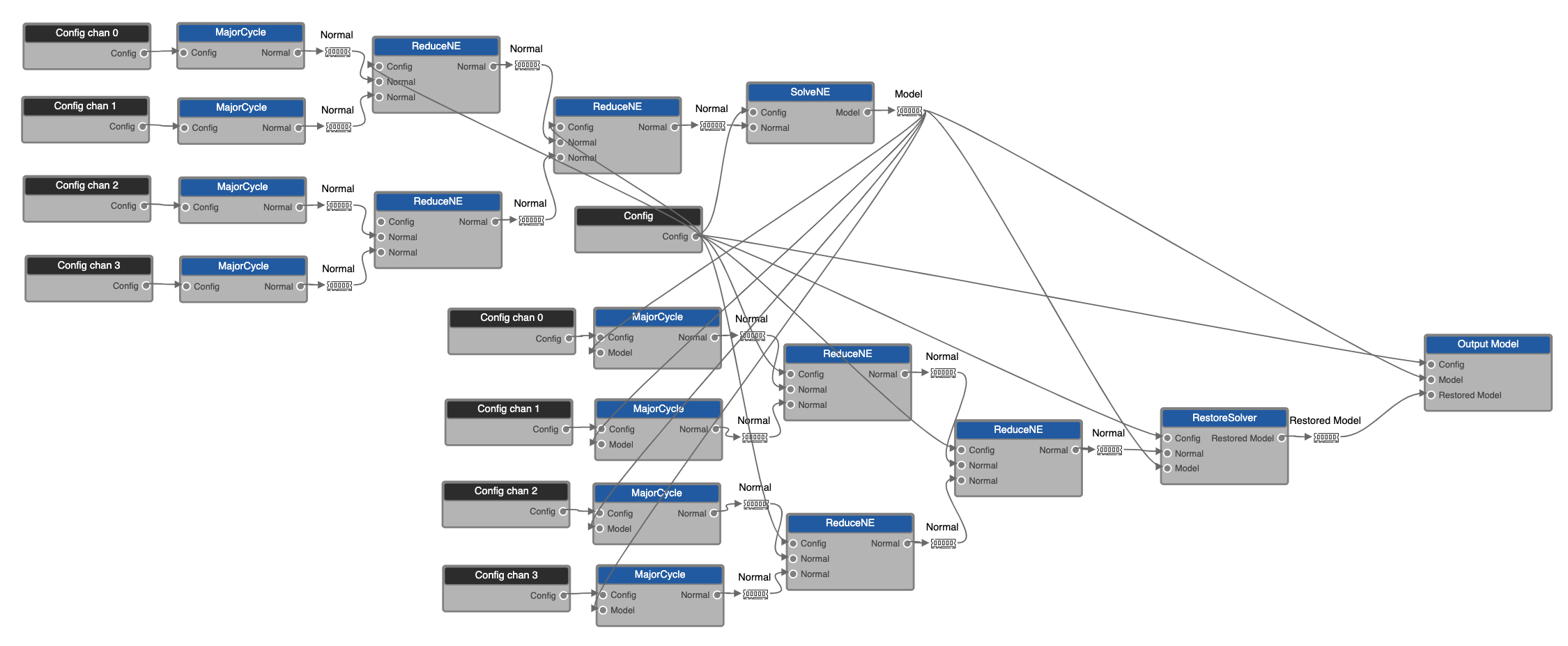
The images being reduced are shown as Normal data drops in the graph, which,
as described below, are BlobString copies of Yandasoft ImagingNormalEquations
objects. These objects contain sets of imaging products, including the main
dirty/residual image hypercube (polarisation, frequency and direction axes),
the PSF hypercube, an alternative PSF hypercube used for preconditioning if
required, and a weights hypercube containing primary beam pixel weights if an
appropriate gridder was used. As the frequencies all have the same image
coordinates, the merging is a simple pixel-wise accumulation. Sky models sent
for prediction and restoring are BlobString copies of Yandasoft Params objects.
These are used throughout Yandasoft calibration and imaging, but in this context
contain just the solved imaging parameters (a clean component hypercube for
each Taylor term) and a small amount of associated metadata. Both of these
classes are defined in the Yandasoft base-scimath library.
On the DALiuGE side, arbitrary parallelism can be achieved using Scatter drops, and multiple major cycle / minor cycle iterations can be realised using a Loop drop. The one feature missing at present is the tree reduction merge, which is implemented in the graph as a series of parallel binary reductions. For N parallel major cycle components, this restricts the depth of reduction to log2N rather than N sucessive merges. A binary tree reduction version of the DALiuGE Gather drop has been earmarked for development in the near future.
One difference between Yandasoft MPI-based parallelism and that of DALiuGE is the independence or otherwise of processes. In Yandasoft, cycling over major and minor cycles is achieved by alternating between parallel major cycle tasks, running on the majority of processes, and the minor cycle tasks running on a single process. Each MPI rank deals with the same set of channels and Taylor terms throughout the imaging process, making it simple and efficient to cache things like visibilities and gridding kernels. However a DALiuGE scatter is set up differently. DALiuGE drops running on a given node either all use the same process space or all use different ones. This makes it hard to cache data between cycles, however it is the more general and flexible approach from a large-scale HPC perspective, where fixing data to specific nodes may not be the optimal solution. An approach better suited to DALiuGE would be to use data drops for persistant data, with the framework deciding what can be cached and what needs to be moved between compute nodes. The partitioning and interfaces described on this page will evolve as JACAL moves in this direction.
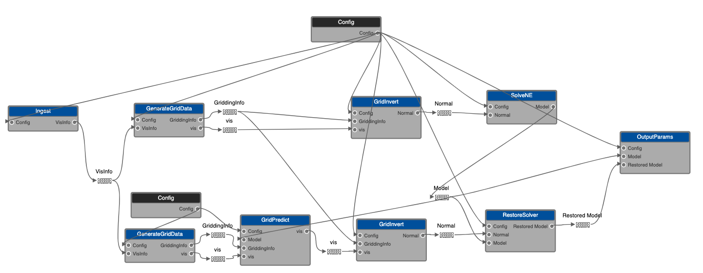
Separate Major Cycle Drops
The main components of the major cycle have been separated out as separate drops.
Ingest: Read data from measurement set and fill a VisInfo partition, including the generation of a visibility data cache.
GenerateGridData: Convert VisInfo partition into a GriddingInfo partition, including the generation of gridding kernel cache. Can be distinct for different types of gridders (e.g. gridders in GridInvert and degridders in GridPredict).
GridInvert: Grid data and weights to form dirty and PSF images.
GridPredict: Degrid model images to form model visibilities, which are subtracted from input visibilities to form output residual visibilities.
An expanded version of the example graph from the EAGLE Usage section is given below.
Yandasoft Data Classes
ImagingNormalEquations
Yandasoft base-scimath ImagingNormalEquations contain the products
generated in the imaging
process. A given object can contain multiple sets of products, which may be
related to one another (such as Taylor term images) or may be entirely
indpendent (although multiple independent imaging paths are not supported in
JACAL). The names of the equations determine the relationship. Each
equation contains the main dirty image hypercube, which may have additional
axes for polarisation and frequency, the PSF hypercube, an alternative PSF
hypercube used for preconditioning if required, and a weights hypercube
containing primary beam pixel weights if an appropriate gridder was used.
Depending on the imaging parameters, the shape, coordinates and reference
pixel may also be stored.
The ImagingNormalEquations class also contains a number of functions for
manipulating data. Of most relevance here is the merge() function. When
one set of equations is merged into another, any equation with a distinct name
is stored separately, however any equations with the same name are combined.
If they have the same shape and coordinates, the various cubes are simply
added together. If the shape or coordinates are different, as they would be
for multi-beaming or facets, accumulation occurs after the image cubes have
been weighted by the weights cubes and reprojected to common coordaintes.
Params
Yandasoft base-scimath Params are used throughout Yandasoft calibration and
imaging as arbitrary containers for both fixed and free parameters. In the
context of imaging, they contain the imaging parameters (i.e. images or
hypercubes) that can be read in from a FITS or CASA image and/or generated
from clean components during deconvolution. In continuum imaging there is a
separate parameter for each Taylor term. Params also contain a small amount
of metadata for each parameter, and a number of functions for manipulating the
metadata. These give a minimal description of the axes of the parameter (type
and extent) and whether or not it is a free parameter. The latter is used, for
example, in auto-differentiation when setting up normal equations.
JACAL Data Classes
A set of new data classes have been added to JACAL to give more flexibility to how data are gridded and degridded. As such, a number of the Yandasoft gridding classes have been copied into JACAL so they can interface with this class and make use of it. It also provides a lightweight way of swapping from the current underlying Yandasoft data accessors to others, such as Apache Plasma.
GriddingData
This is a simple container to hold one or more VisInfo and/or GriddingInfo objects.
VisInfo
The visibility data ingested by an Ingest process are stored in one or more data partitions of type VisInfo. Current partitioning options are time or w-value, with frequency partitioning handled by the underlying data accessors. However other options can be added in a straightforward manner. The visibilities and metadata are stored as flat vectors and the partitioning tasks deal with any algorithmic complexities. Current vectors are:
int itsNumberOfSamples; // total number of baselines & frequencies in each partition
int itsNumberOfPols; // number of polarisations
int itsNumberOfChannels; // number of frequencies (needed to handle Taylor term weighting)

bool itsConvertedToImagePol; // have the vis and weights been converted to the imaging polarisation frame?

/// Pointing metadata
casacore::MVDirection itsImageCentre;
casacore::MVDirection itsTangentPoint;

/// Vectors of length itsNumberOfSamples
std::vector<double> itsU; // u coordinate in wavelengths. Not used after init.
std::vector<double> itsV; // v coordinate in wavelengths. Not used after init.
std::vector<double> itsW; // w coordinate in wavelengths. Not used after init.
std::vector<std::complex<float> > itsPhasor; // phase shift for each visibility
std::vector<int> itsChannel; // frequency channel, needed to handle Taylor term weighting
std::vector<bool> itsFlag; // flagging state

/// A-projection vectors of length itsNumberOfSamples
std::vector<casacore::MVDirection> itsPointingDir1; // Not used after init.
std::vector<casacore::MVDirection> itsPointingDir2; // Not used after init.
std::vector<float> itFeed1PA; // not used after init.
std::vector<float> itFeed2PA; // not used after init.

/// Vectors of length itsNumberOfPols
casacore::Vector<casacore::Stokes::StokesTypes> itsStokes;

/// Vectors of length itsNumberOfChannels
std::vector<double> itsFrequencyList;

/// Nested vectors of length itsNumberOfSamples,itsNumberOfPols
std::vector<std::vector<float> > itsWeight; // vis sample weight.
std::vector<std::vector<float> > itsNoise; // sample RMS. Not used after init.
std::vector<std::vector<std::complex<float> > > itsSample; // vis samples
GriddingInfo
The GenerateGridData application converts a set of VisInfo partitions to an equal number of GriddingInfo partitions. These metadata are also stored as flat vectors. The gridders are set up to simply grid or degrid the elements of the vectors stored in this class. All data required by the Yandasoft gridders are currently passed in this class, but the gridders and the interface are expected to evolve towards the interface used in the SKA Processing Function Library. The GenerateGridData application also generates the cache of gridding kernels. Current vectors are:
int itsNumberOfSamples; // total number of baselines & frequencies in each partition
int itsNumberOfPols; // number of polarisations
int itsNumberOfChannels; // number of frequencies (needed to handle Taylor term weighting)

/// Vectors of length itsNumberOfSamples
std::vector<std::complex<float> > itsPhasor; // phase shift for each visibility
std::vector<int> itsChannel; // frequency channel, needed to handle Taylor term weighting
std::vector<bool> itsFlag; // flagging state
std::vector<int> itsGridIndexU; // u index in grid
std::vector<int> itsGridIndexV; // v index in grid
std::vector<int> itsKernelIndex; // index in kernel grid, including oversampling planes

/// Vectors of length itsNumberOfChannels
std::vector<double> itsFrequencyList;

/// Nested vectors of length itsNumberOfSamples,itsNumberOfPols
std::vector<std::vector<float> > itsWeight; // vis sample weight.

/// Convolution kernels
int nPlanes;
std::vector<int> cSize; // Vector of kernel sizes (length nPlanes)
std::vector<std::vector<casacore::Complex> > itsConvFunc; // Nested vector of kernels ([nPlanes][cSize*cSize])
std::vector<std::vector<int> > itsConvFuncOffsets; // Nested vector of kernel offsets ([nPlanes][2])
JACAL Interfaces
Interfaces between JACAL imaging components are at present data drops formed from Yandasoft and JACAL classes that have been converted to BlobStrings.
ImagingNormalEquations
/// @brief write the object to a blob stream
void ImagingNormalEquations::writeToBlob(LOFAR::BlobOStream& os) const
{
  os << itsNormalMatrixSlice // PSF cubes; dirty image cubes; std::map<std::string, casacore::Vector<imtype> >
     << itsNormalMatrixDiagonal // weights cubes; dirty image cubes; std::map<std::string, casacore::Vector<imtype> >
     << itsPreconditionerSlice // dirty image cubes; std::map<std::string, casacore::Vector<imtype> >
     << itsShape // shape of the cubes; std::map<std::string, casacore::IPosition>
     << itsReference // reference pixel of images; std::map<std::string, casacore::IPosition>
     << itsCoordSys // coordinate system of the images; std::map<std::string, casacore::CoordinateSystem>
     << itsDataVector; // dirty image cubes; std::map<std::string, casacore::Vector<imtype> >
}

/// @brief read the object from a blob stream
void ImagingNormalEquations::readFromBlob(LOFAR::BlobIStream& is)
{
  is >> itsNormalMatrixSlice
     >> itsNormalMatrixDiagonal
     >> itsPreconditionerSlice
     >> itsShape
     >> itsReference
     >> itsCoordSys
     >> itsDataVector;
}
Type imtype is either float or double.
Params
/// @brief write the object to a blob stream
LOFAR::BlobOStream& operator<<(LOFAR::BlobOStream& os, const Params& par)
{
    os.putStart("Params",BLOBVERSION);
    os << par.itsUseFloat // use float or double for the Arrays; bool
       << par.itsArrays // image data; std::map<std::string, casacore::Array<double> >
       << par.itsArraysF // image data; std::map<std::string, casacore::Array<float> >
       << par.itsAxes // image axes; std::map<std::string, Axes>
       << par.itsFree; // the free/fixed status of the parameter; std::map<std::string, bool>
    os.putEnd();
    return os;
}

/// @brief read the object from a blob stream
LOFAR::BlobIStream& operator>>(LOFAR::BlobIStream& is, Params& par)
{
    const int version = is.getStart("Params");
    ASKAPCHECK(version == BLOBVERSION, "Attempting to read from a blob stream of the wrong version");
    is >> par.itsUseFloat
       >> par.itsArrays
       >> par.itsArraysF
       >> par.itsAxes
       >> par.itsFree;
    is.getEnd();
    // as the object has been updated one needs to obtain new change monitor
    par.itsChangeMonitors.clear();
    return is;
}
Type Axes is also defined in the Yandasoft base-scimath library. It contains the
names (e.g. “RA_LIN”, “FREQ”) and extrema (start and end values as doubles) of
a set of axes, using standard casacore types such as
casacore::DirectionCoordinate and casacore::Stokes::StokesTypes.
GriddingInfo
/// @brief write the object to a blob stream
LOFAR::BlobOStream& operator<<(LOFAR::BlobOStream& os, const GriddingInfo& info)
{
    // Copy the cache of gridding kernels to a suitable format.
    // This will be removed once a final cache format has been chosen.
    const int nPlanes = info.itsConvFunc.size();
    std::vector<int> cSize(nPlanes);
    std::vector<std::vector<casacore::Complex> > tmpConvFunc(nPlanes);
    for (uint plane = 0; plane < nPlanes; ++plane) {
        cSize[plane] = info.itsConvFunc[plane].nrow();
        tmpConvFunc[plane].resize(cSize[plane]*cSize[plane]);
        for (uint j = 0; j < cSize[plane]; ++j) {
            for (uint i = 0; i < cSize[plane]; ++i) {
                tmpConvFunc[plane][j*cSize[plane]+i] = info.itsConvFunc[plane](i,j);
            }
        }
    }
    os.putStart("GriddingInfo",BLOBVERSION);
    os << info.itsNumberOfSamples
       << info.itsNumberOfChannels
       << info.itsNumberOfPols
       << info.itsFrequencyList
       << info.itsGridIndexU
       << info.itsGridIndexV
       << info.itsKernelIndex
       << info.itsPhasor
       << info.itsChannel
       << info.itsFlag
       << info.itsWeight
       << nPlanes
       << cSize
       << tmpConvFunc;
    os.putEnd();
    return os;
}
/// @brief read the object from a blob stream
LOFAR::BlobIStream& operator>>(LOFAR::BlobIStream& is, GriddingInfo& info)
{
    const int version = is.getStart("GriddingInfo");
    ASKAPCHECK(version == BLOBVERSION, "Attempting to read from a blob stream of the wrong version");
    // first get size parameters and resize the vectors
    is >> info.itsNumberOfSamples
       >> info.itsNumberOfChannels
       >> info.itsNumberOfPols;
    is >> info.itsFrequencyList
       >> info.itsGridIndexU
       >> info.itsGridIndexV
       >> info.itsKernelIndex
       >> info.itsPhasor
       >> info.itsChannel
       >> info.itsFlag
       >> info.itsWeight;
    int nPlanes;
    is >> nPlanes;
    std::vector<int> cSize(nPlanes);
    is >> cSize;
    std::vector<std::vector<casacore::Complex> > tmpConvFunc(nPlanes);
    for (uint plane = 0; plane < nPlanes; ++plane) {
        tmpConvFunc[plane].resize(cSize[plane]*cSize[plane]);
    }
    is >> tmpConvFunc;
    // Copy the cache of gridding kernels back to the required format.
    // This will be removed once a final cache format has been chosen.
    info.itsConvFunc.resize(nPlanes);
    for (uint plane = 0; plane < nPlanes; ++plane) {
        info.itsConvFunc[plane].resize(cSize[plane],cSize[plane]);
        for (uint j = 0; j < cSize[plane]; ++j) {
            for (uint i = 0; i < cSize[plane]; ++i) {
                info.itsConvFunc[plane](i,j) = tmpConvFunc[plane][j*cSize[plane]+i];
            }
        }
    }
    is.getEnd();
    return is;
}
vis data
The GenerateGridData application extracts the visibility data and passes them as a separate blob drop. The current format, which is expected to change, is a simple nested vector of complex values:
std::vector<std::vector<std::complex<float> > > vis;
vis.resize(itsNumberOfSamples);
for (uint i=0; i<itsNumberOfSamples; ++i) {
    vis[i].resize(itsNumberOfPols);
}